The moments of this distribution are the cogrowth sequence of the lamplighter group

Group Theory

The lamplighter group is defined as the wreath product $L:=\mathbb Z_2 \wr \mathbb Z$ and has the standard presentation $L=\langle a,t : a^2, (at^nat^{-n})^2,\, n\in \mathbb Z\rangle$. The group has a nice mental image: imagine a lamppost at every integer and a “lamplighter” that can walk between lights and turn them on and off. The generator $a$ is “toggle the light you’re at” and the generator $t$ is ``move one to the right’’. The first relation says that toggling a light on and then off (or vice versa) returns you to the previous state. The second relation says that turning a light on, moving $n$ to the right, turning that light on, and then going back to where you started is an order two “action”. Doing this again clearly just reverses what you already did.

The lamplighter group is very heavily studied. Of particular interest are the growth and cogrowth rate of the group. Let $a_n$ denote the number of non-identity elements one can form as a product of $n$ generators, this is called the growth sequence. Similarly, $b_n$ will denote the number of ways one can combine $n$ generators to get the identity, this is called the cogrowth sequence. The authors in [PrGu17] computed the cogrowth sequence up to a large cutoff by a polynomial-time algorithm. Their data can be found on the OEIS, which is where I originally discovered this connection. The cogrowth sequence of this group is nice to think about: starting at $0$, how many ways can you make $n$ moves (either moving one step or toggling a light) such that you return to the origin and don’t leave any lights on? Combinatorially, this is the number of returning walks on the integers such that, if you “lazy step” on any given number, you must do so an even number of times throughout the walk.

Random Matrix Theory

Let $C_n$ denote the cycle graph on $n$ vertices and $A_{C_n}$ its adjacency matrix. Let $D_n$ be a diagonal matrix with entries i.i.d. Rademacher random variables, uniform over ${-1,1}.$ We want to consider the sequence of random matrices given by $C_n+D_n$. Since the eigenvalues of these random matrices are randomly distributed, we may ask about their distribution. In fact, for many ensembles of random matrices, the distribution of eigenvalues (or empirical spectral distribution) converges to some smooth distribution (the limiting spectral distribution), as the matrix size $n\to \infty$, with high probability [Tao11].

For the purpose of our discussion, let $A_n\in \mathbb{R}^{n\times n}$ be a sequence of nice symmetric matrices (think of them as having Gaussian or smooth entries satisfying some independence). The eigenvalues are real and the moments of the limiting distribution can be computed as limits of traces of powers of the matrix in question. Since the entries and eigenvalues are random, we have a distribution of distributions and we can only compute moments in expectation. The expected value of the $k^{th}$ moment of the $n^{th}$ matrix is
\begin{equation} \mathbb{E}\mu_{k,n} = \frac{1}{n} \mathbb{E} \sum_{i=1}^n \lambda^k= \frac{1}{n}\mathbb{E}\mathrm{Tr}(A_n^k). \end{equation}

This trace can be split as a sum over cyclic products of matrix entries: \begin{equation} \mathbb{E} \mathrm{Tr}(A_n^k) = \sum_{i_1,i_2,\dots, i_k} \mathbb{E}[A_n(i_1,i_2)A_n(i_2,i_3)\dots A_n(i_{k-1},i_k)A_n(i_ki_1)]. \end{equation} Let’s now return to the case of $A_n= A_{C_n}+D_n$ where we can rephrase this trace combinatorially. Since we take expectation, we need to be careful about which terms contribute. If the pairs $(i_j,i_{j+1})$ are distinct, we don’t have to worry about the expectation since each of the off-diagonal entries are in the set ${0,1}$. For a term to contribute, all we need is that vertex $i_j$ is connected to vertex $i_{j+1}$ for all $j$; these contribute if and only if the vertex sequence is a returning path, with no lazy steps, on the n-cycle.

The Rademacher random variables have odd moments $0$ and all even moments are equal to $1$. If some $i_{j_1}=i_{j_2}$, we need an even number of such occurrences for the expectation to be nonzero, and these expectations multiply the term by $1$. We see a similarity between these traces and the combinatorial problem associated to the lamplighter group, there’s just one hangup. Since we’re dealing with the cycle, what if paths wrap around somehow? We can rest easy in the limit, since, as $n\to \infty$, the size of the cycle goes to infinity while, in the fixed moment we’re computing, the path lengths are constant.

Immediately, we see that there are no odd-length paths so the odd moments are $0$ and we should have a symmetric limiting distribution (at least in expectation).

Some Visualizations

Plotting the histogram of eigenvalues for $1000$ samples of $A_{3000}$, we get the following interesting shape.

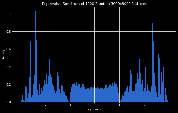
The moments we get numerically here match closely with the cogrowth sequence of the lamplighter group. The computed even moments are approximately [3,15,87,547,3623,…] before they diverge from the expected sequence.

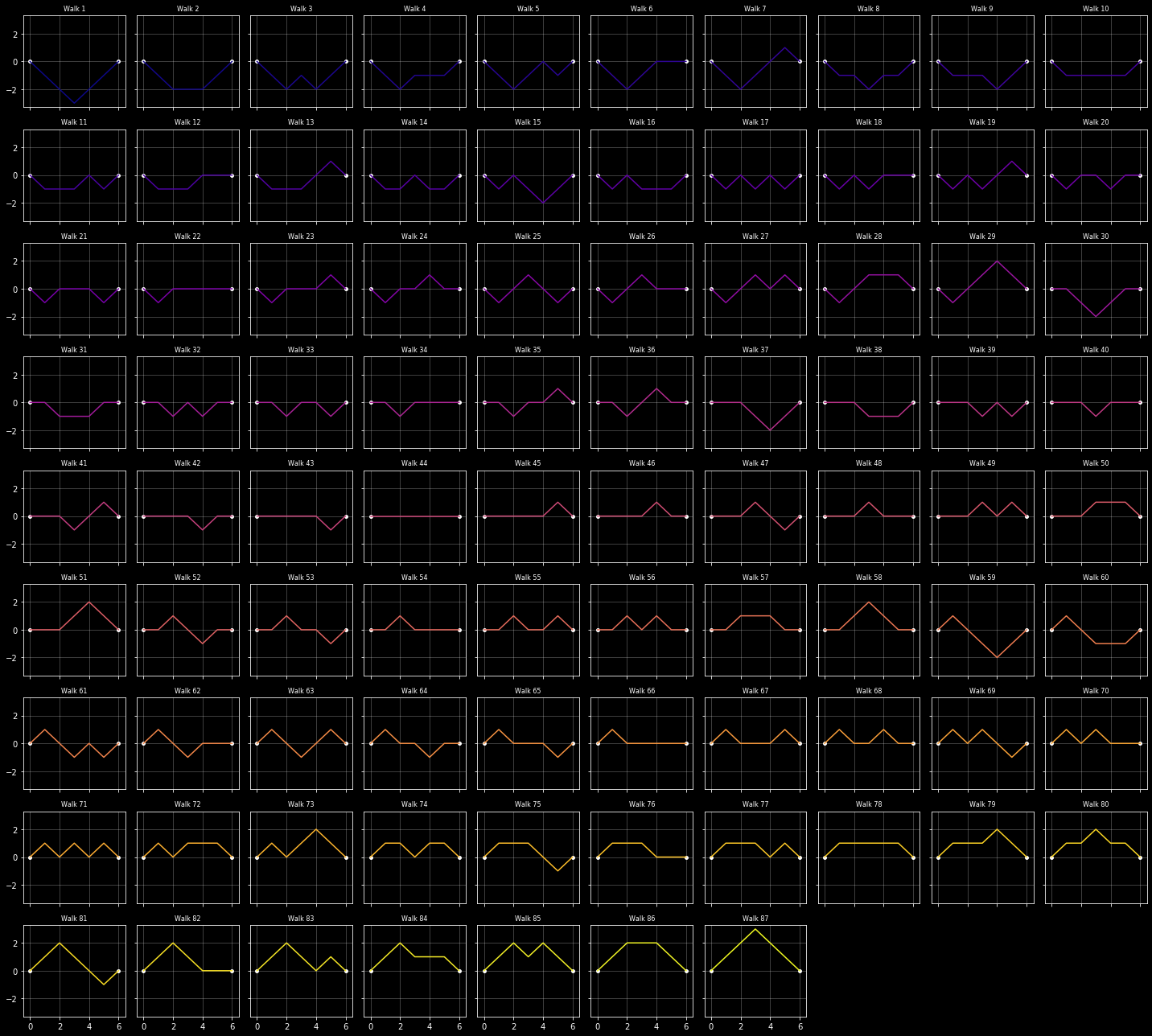
It’s also fun to enumerate all of the paths of a given length. Here are the 87 paths of length 6.

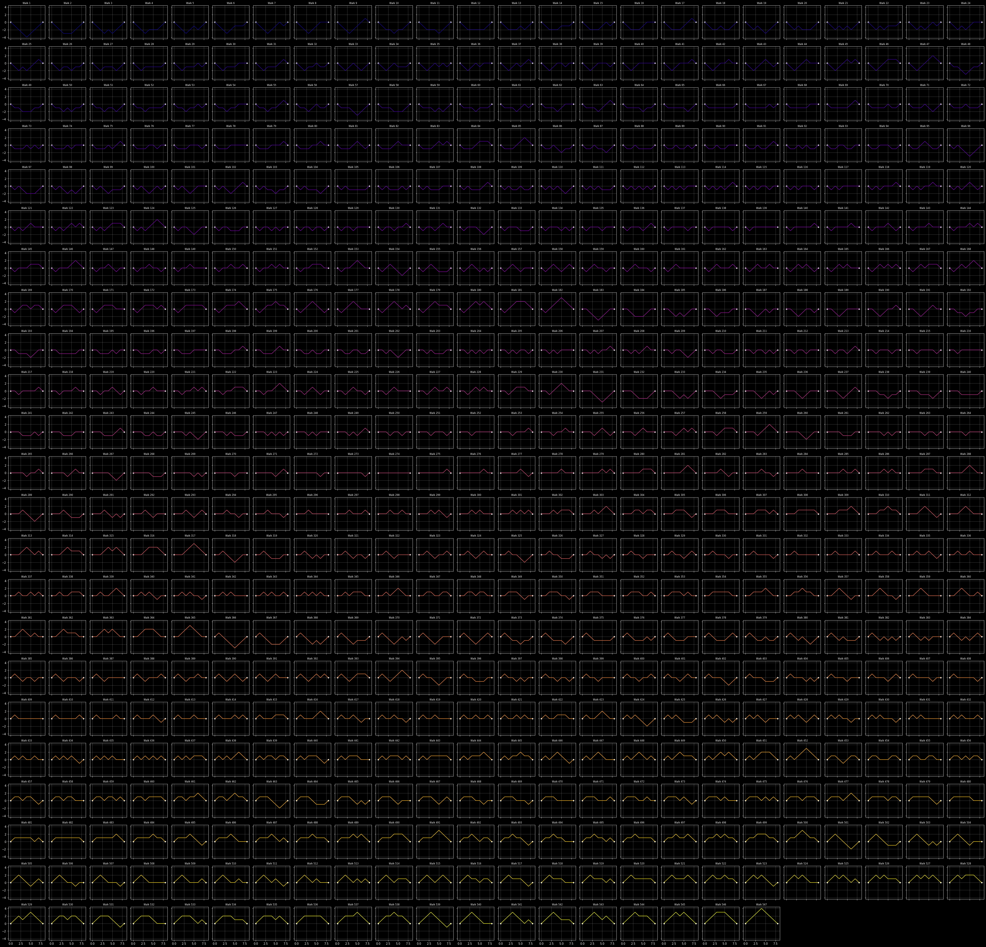
For higher lengths, the number of valid walks increases quite quickly so we have to visualize them differently. Here are all of the paths of length $8$ overlaid on a plot

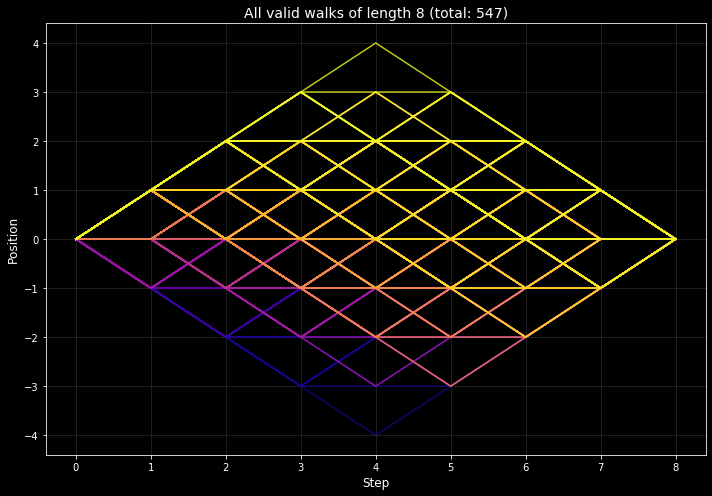
and here are the same paths presented sequentially as an animation.

For the full grid of paths of length 8, click here and for paths of length 10 click here.

Proving It

To formalize all of this, one needs to show that the moments converge not just in expectation, but with high probability. We’ll need the following result,

Lemma. (McDiarmid’s Inequality) Let $f: \mathcal{X}_1\times \mathcal{X}_2 \times \cdots \times \mathcal{X}_n \to \mathbb{R}$. Assume that changing the value of $x_i$ changes the value of $f$ by at most $c_i$. Let $X_1,X_2,\dots, X_n$ be independent random variables with $X_i\in \mathcal{X}_i$ for all $i$, then

\begin{equation} P(\lvert f(X_1,X_2,\dots, X_n)- \mathbb{E}[f(X_1,X_2,\dots, X_n)] \rvert \geq \varepsilon ) \leq 2\mathrm{exp}\left( -\frac{2\varepsilon^2}{\sum c_i^2}\right). \end{equation}

This result is proved in [McD89].

Theorem. Let $\mu_k(A_n)$ denote the $k^{th}$ moment of the empirical spectral distribution of the matrix $A_n$. With high probability, we have $\lim_{n\to\infty} \mu_k(A_n)=b_k$, where ${b_k}$ denotes the cogrowth sequence of the lamplighter group.

Proof. We have already argued that this holds in expectation, so it suffices to make some concentration argument. Thankfully, this is doable with crude bounding.

Fix $k, N\in \mathbb{N}$. The value $\mu_k(A_n)$ is a random variable dependent on the diagonal Rademacher random variables. Hence, it can be viewed as a function, with abuse of notation, $\mu_k(A_n): {-1,1}^n\to \mathbb{R}$ . We want to understand how much the moment changes if we flip one coordinate from $1$ to $-1$ or vice versa. Recall that we have \begin{equation} \mathrm{Tr}(A_n^k) = \sum_{i_1,i_2,\dots, i_k} A_n(i_1,i_2)A_n(i_2,i_3)\dots A_n(i_{k-1},i_k)A_n(i_ki_1). \end{equation}

We now roughly bound the number of terms in this sum in which $A(i,i)$ appears for some fixed $1\leq i\leq n$. We always assume $n\gg k$, so that the number of valid walks on the cycle starting from a fixed vertex is equal to the number of valid walks on the integers starting at 0. A priori, the number of valid walks depends on $n$ since we may freely choose the base-point. Once we enforce that our path must visit $A(i,i)$, however, the dependence on $n$ disappears. This is because the path may start at most $k/2$ vertices away from $A(i,i)$ and so we have but $k$ choices of base point. There are $k$ choices of base point and $k-1$ free moves each with three options, so $A(i,i)$ appears in at most $k3^{k-1}$ terms in the trace sum.

Since each term of the trace sum takes a value in ${-1,0,1}$, flipping the value of the $i^{th}$ coordinate changes the value of $\mathrm{Tr}(A_n^k)$ by at most $k3^{k-1}$. After normalizing by $1/n$ (we’re taking the average over $n$ eigenvalues), we see that flipping the $i^{th}$ coordinate changes the value of $\mu(A_n^k)$ by at most $\frac{k3^{k-1}}{n}$.

Applying McDiarmid’s Inequality for $c_i= \frac{k3^{k-1}}{n}$ for all $i$, we see

\begin{equation} P(\lvert \mu_k(A_n)- \mathbb{E}[\mu_k(A_n)] \rvert \geq \varepsilon ) \leq 2\mathrm{exp}\left( -\frac{2\varepsilon^2n}{k3^{k-1}}\right) \end{equation} which vanishes as $n\to \infty$, completing the proof.

References

[PrGu17] Numerical studies of Thompson’s group F and related groups, Andrew Elvey Price and Anthony J Guttmann, 2017. URL: arXiv

[Tao11] Topics in random matrix theory, Terrance Tao, 2011. URL: Tao’s Blog

[McD89] McDiarmid, Colin (1989). “On the method of bounded differences”. Surveys in Combinatorics, 1989: Invited Papers at the Twelfth British Combinatorial Conference: 148–188.